Using Convolution to Generalize
Convolutions
Convolutions deliver locality and translation invariance
- If we want to recognize patterns corresponding to objects, we will likely need to look at how nearby pixels are arranged, and we will be less interested in how pixels that are far from each other appear in combination.
- In order to translate this intuition into mathematical form, we could compute the weighted sum of a pixel with its immediate neighbors, rather than with all other pixels in the image.
What convolutions do
Translation invariant: we want these localized patterns to have an effect on the output regardless of their location in the image.
Convolution is defined for a 2D image as the scalar product of a weight matrix, the kernel, with every neighborhood in the input. The following figure illustrates applying a 3x3 kernel on a 2D image:
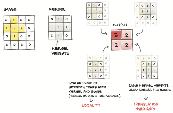
- The weights in the kernel are NOT known in advance, but they are initialized randomly and updated through backpropagation.
- It is the SAME kernel, and thus each weight in the kernel, is reused across the whole image.
- Thinking back to autograd, this means the use of each weight has a history spanning the entire image. Thus, the derivative of the loss with respect to a convolution weight includes contributions from the entire image.
Summarizing, by using to convolutions, we get
- Local operations on neighborhoods 👏
- Translation invariance 👏
- Models with a lot fewer parameters 👏
- With a convolution layer, the number of parameters depends on
- the size of the convolution kernel (3x3, 5x5, and so on)
- how manyy convlution filters (or output channels) we decide to use in our model.
- With a convolution layer, the number of parameters depends on
Convolutions in PyTorch
The torch.nn module provides convolutions for 1, 2, and 3 dimensions:
nn.Conv1dfor time seriesnn.Conv2dfor imagesnn.Conv3dfor volumes or videos
For image data, we will use nn.Conv2d. The arguments we provide to nn.Conv2d are
the number of input features/channels (since we’re dealing with multichannel images: that is, more than one value per pixel)
the number of output features
the size of the kernel
It is very common to have kernel sizes that are the same in all directions, so PyTorch has a shortcut for this: whenever
kernel_size=3is specified for a 2D convolution, it means 3 × 3 (provided as a tuple (3, 3) in Python).
For example:
in_ch = 3 # 3 input features epr pixel (the RGB channels)
out_ch = 16 # arbitrary number of channels in the output

conv = nn.Conv2d(in_ch, out_ch, kernel_size=3)
conv
Conv2d(3, 16, kernel_size=(3, 3), stride=(1, 1))
In addition, we need to add the zeroth batch dimension with unsqueeze if we want to call the conv module with one input image, since nn.Conv2d expects a B × C × H × W shaped tensor as input:
# cifar2 is a modified cifar10 which contains only airplanes and birds

img, _ = cifar2[0]
output = conv(img.unsqueeze(dim=0))
img.unsqueeze(0).shape, output.shape
(torch.Size([1, 3, 32, 32]), torch.Size([1, 16, 30, 30]))
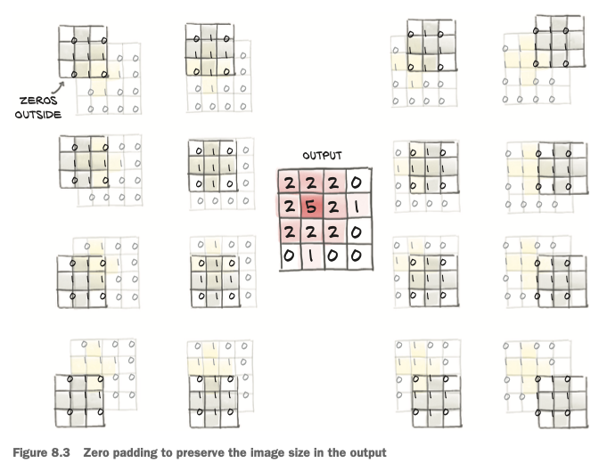
Padding the boundary
By default, PyTorch will slide the convolution kernel within the input picture, getting width - kernel_width + 1 horizontal and vertical positions. PyTorch gives us the possibility of padding the image by creating ghost pixels around the border that have value zero as far as the convolution is concerned.
conv = nn.Conv2d(3, 1, kernel_size=3, padding=1)
output = conv(img.unsqueeze(0))
img.unsqueeze(0).shape, output.shape
(torch.Size([1, 3, 32, 32]), torch.Size([1, 1, 32, 32]))
🤔 Reasons to pad convolutions
- Doing so helps us separate the matters of convolution and changing image sizes, so we have one less thing to remember
- when we have more elaborate structures such as skip connections or the U-Nets, we want the tensors before and after a few convolutions to be of compatible size so that we can add them or take differences.
Detecting features with convolutions
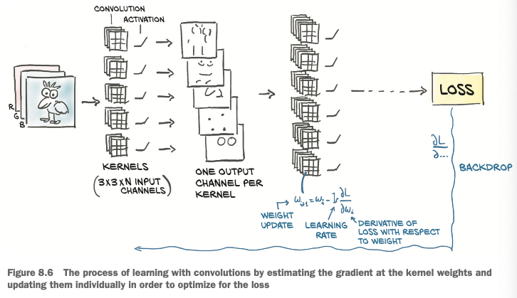
With deep learning, we let kernels be estimated from data in whatever way the discrimination is most effective. The the job of a convolutional neural network is to estimate the kernel of a set of filter banks in successive layers that will transform a multichannel image into another multichannel image, where different channels correspond to different features (such as one channel for the average, another channel for vertical edges, and so on).
The following figure shows how the training automatically learns the kernels:
Pooling
From large to small: downsampling
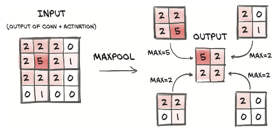
Max pooling: taking non-overlapping 2 x 2 tiles and taking the maximum over each of them as the new pixel at the reduced scale.
💡 Intuition of max pooling:
The output images from a convolution layer, especially since they are followed by an activation just like any other linear layer, tend to have a high magnitude where certain features corresponding to the estimated kernel are detected (such as vertical lines). By keeping the highest value in the 2 × 2 neighborhood as the downsampled output, we ensure that the features that are found survive the downsampling, at the expense of the weaker responses.
Max pooling is provided by the nn.MaxPool2d module. It takes as input the size of the neighborhood over which to operate the pooling operation. If we wish to downsample our image by half, we’ll want to use a size of 2.
pool = nn.MaxPool2d(2)
output = pool(img.unsqueeze(dim=0))

img.unsqueeze(0).shape, output.shape
(torch.Size([1, 3, 32, 32]), torch.Size([1, 3, 16, 16]))
Combining convolutions and downsampling
Combining convolutions and downsampling can help us recognize larger structures
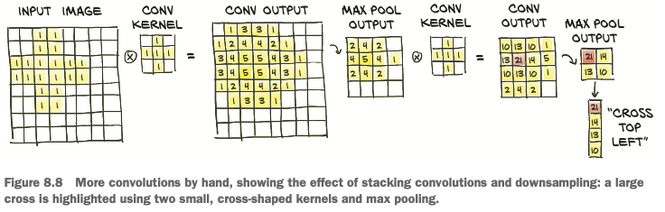
- we start by applying a set of 3 × 3 kernels on our 8 × 8 image, obtaining a multichannel output image of the same size.
- Then we scale down the output image by half, obtaining a 4 × 4 image, and apply another set of 3 × 3 kernels to it.
- The second set of kernels
- operates on a 3 × 3 neighborhood of something that has been scaled down by half, so it effectively maps back to 8 × 8 neighborhoods of the input.
- takes the output of the first set of kernels (features like averages, edges, and so on) and extracts additional features on top of those.
Summarizing up:
- the first set of kernels operates on small neighborhoods on first-order, low-level features,
- while the second set of kernels effectively operates on wider neighborhoods, producing features that are compositions of the previous features.
This is a very powerful mechanism that provides convolutional neural networks with the ability to see into very complex scenes 💪
Subclassing nn.Module
In order to subclass nn.Module
- we need to define a
forwardfunction that takes the inputs to the module and returns the output. (This is where we define our module’s computation.)- With PyTorch, if we use standard torch operations,
autogradwill take care of the backward pass automatically 👏; and indeed, annn.Modulenever comes with abackward.
- With PyTorch, if we use standard torch operations,
- To use other submodules (premade like convolutions or cutomized), we typically define them in the constructor
__init__and assign them to self for use in theforwardfunction. Before we can do that, we need toc allsuper().__init__()
For example, let’s model the following network:
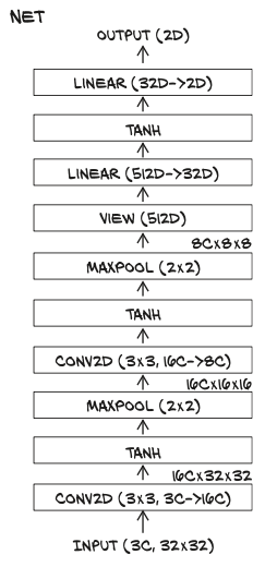
class Net(nn.Module):

    def __init__(self):
        super().__init__()

        self.conv1 = nn.Conv2d(3, 16, kernel_size=3, padding=1)
        self.act1 = nn.Tanh()
        self.pool1 = nn.MaxPool2d(2)

        self.conv2 = nn.Conv2d(16, 8, kernel_size=3, padding=1)
        self.act2 = nn.Tanh()
        self.pool2 = nn.MaxPool2d(2)

        self.fc1 = nn.Linear(8 * 8 * 8, 32)
        self.act3 = nn.Tanh()
        self.fc2 = nn.Linear(32, 2)

    def forward(self, x):
        out = self.pool1(self.act1(self.conv1(x)))
        out = self.pool2(self.act2(self.conv2(out)))

        # we leave the batch dimension as –1 in the call to view,
        # since in principle we don’t know how many samples will be in the batch.
        out = out.view(-1, 8 * 8 * 8)

        out = self.act3(self.fc1(out))
        out = self.fc2(out)

        return out
Keep track of parameters and submodules
Assigning an instance of nn.Moduleto an attribute in an nn.Module automatically registers the module as a submodule. We can call arbitrary methods of an nn.Module subclass.
We can call arbitrary methods of an nn.Module subclass. This allows Net to have access to the parameters of its submodules without further action by the user:
model = Net()

numel_list = [p.numel() for p in model.parameters()]
sum(numel_list), numel_list
(18090, [432, 16, 1152, 8, 16384, 32, 64, 2])
The functional API
Looking back at the implementation of the Net class, it appears a bit of a waste that we are also registering submodules that have no parameters, like nn.Tanh and nn.MaxPool2d. It would be easier to call these directly in the forward function, just as we called view.
PyTorch has functional counterparts for every nn module.
By “functional” here we mean “having no internal state”—in other words, “whose output value is solely and fully determined by the value input arguments.”
torch.nn.functional provides many functions that work like the modules we find in nn . Instead of working on the input arguments and stored parameters like the module counterparts, they take inputs and parameters as arguments to the function call. For instance, the functional counterpart of nn.Linear is nn.functional.linear, which is a function that has signature linear(input, weight, bias=None). The weight and bias parameters are arguments to the function.
Let’s switch to the functional counterparts of pooling and activation, since they have no parameters:
import torch.nn.functional as F

class Net(nn.Module):

    def __init__(self):
        super().__init__()
        self.conv1 = nn.Conv2d(3, 16, kernel_size=3, padding=1)
        self.conv2 = nn.Conv2d(16, 8, kernel_size=3, padding=1)
        self.fc1 = nn.Linear(8 * 8 * 8, 32)
        self.fc2 = nn.Linear(32, 2)

    def forward(self, x):
        out = F.max_pool2d(torch.tanh(self.conv1(x)), 2)
        out = F.max_pool2d(torch.tanh(self.conv2(out)), 2)
        out = out.view(-1, 8 * 8 * 8)
        out = torch.tanh(self.fc1(out))
        out = self.fc2(out)
        return out
Training the convnet
Two nested loops:
- an outer one over the epochs and
- an inner one of the
DataLoaderthat produces batches from ourDataset. In each loop, we then have to- Feed the inputs through the model (the forward pass).
- Compute the loss (also part of the forward pass).
- Zero any old gradients.
- Call
loss.backward()to compute the gradients of the loss with respect to all parameters (the backward pass). - Have the optimizer take a step in toward lower loss.
- an inner one of the
import datetime

def training_loop(n_epochs, optimizer, model, loss_fn, train_loader):
    for epoch in range(1, n_epochs+1):
        loss_train = 0.0
        for imgs, labels in train_loader:

            # feeds a batch through our model
            outputs = model(imgs)

            # computes the loss we wish to minimize
            loss = loss_fn(outputs, labels)

            # get rid of the gradients from the last round
            optimizer.zero_grad()

            # perform the backward step
            # (we compute the gradients of all parameters we want the network to learn)
            loss.backward()

            # update the model
            optimizer.step()

            # sum the losses over the epoch
            loss_train += loss.item() # use .item() to escape the gradients

        if epoch == 1or epoch % 10 == 0:
            print(f'{datetime.datetime.now()}: '
            f'Epoch {epoch}, Training loss: {loss_train / len(train_loader)}')
train_loader = torch.utils.data.DataLoader(cifar2, batch_size=64, shuffle=True)
model = Net()
optimizer = optim.SGD(model.parameters(), lr=1e-2)
loss_fn = nn.CrossEntropyLoss()

training_loop(n_epochs=100, optimizer=optimizer, model=model, loss_fn=loss_fn,
              train_loader=train_loader)
Measuring accuracy
Measure the accuracies on the training set and validation set:
train_loader = torch.utils.data.DataLoader(cifar2, batch_size=64, shuffle=False)
val_loader = torch.utils.data.DataLoader(cifar2_val, batch_size=64, shuffle=False)

def validate(model, train_loader, val_loader):
    for name, loader in [("train", train_loader), ("val", val_loader)]:
        correct, total = 0, 0
        with torch.no_grad():
            for imgs, labels in loader:
                outputs = model(imgs)
                _, predicted = torch.max(outputs, dim=1)
                total += labels.shape[0]
                correct += int((predicted == labels).sum())

        print(f'Accuracy {name} : {(correct / total):.2f}')

validate(model, train_loader, val_loader)
Saving and loading model
Save the model to a file:
# assume that the data_path is already specified
# and we want to save our model with the name "birds_vs_airplanes.pt"

torch.save(model.state_dict(), data_path + 'birds_vs_airplanes.pt')
The birds_vs_airplanes.pt file now contains all the parameters of model: weights and biases for the two convolution modules and the two linear modules. No structure, just the weights.
When we deploy the model in production, we’ll need to keep the model class handy, create an instance, and then load the parameters back into it:
loaded_model = Net()
loaded_model.load_state_dict(torch.load(data_path + 'birds_vs_airplanes.pt'))
<All keys matched successfully>
Training on GPU
nn.Module implements a .to function that moves all of its parameters to the GPU (or casts the type when you pass a dtype argument). There is a somewhat subtle difference between Module.to and Tensor.to.
Module.tois in place: the module instance is modified.- But
Tensor.tois out of place (in some ways computation, just like Tensor.tanh), returning a new tensor.
📝 Good practice:
create the
Optimizerafter moving the parameters to the appropriate devicemove things to the GPU if one is available. A good pattern is to set the a variable device depending on
torch.cuda.is_available:device = (torch.device('cuda') if torch.cuda.is_available() else torch.device('cpu'))
Let’s amend the training loop by moving the tensors we get from the data loader to the GPU by using the Tensor.to method.
import datetime

def training_loop(n_epochs, optimizer, model, loss_fn, train_loader):
    for epoch in range(1, n_epochs + 1):
        loss_train = 0.0

        for imgs, labels in train_loader:

            # Move imgs and labels tensors to the device we're training on
            imgs = imgs.to(device=device)
            labels = labels.to(device=device)

            outputs = model(imgs)

            loss = loss_fn(outputs, labels)

            optimizer.zero_grad()
            loss.backward()
            optimizer.step()

            loss_train += loss.item()

        if epoch == 1or epoch % 10 == 0:
            print(f'{datetime.datetime.now()}: '
            f'Epoch {epoch}, Training loss: {loss_train / len(train_loader)}')
Now we can instantiate our model, move it to device, and run it:
(Note: If you forget to move either the model or the inputs to the GPU, you will get errors about tensors not being on the same device, because the PyTorch operators do not support mixing GPU and CPU inputs.)
train_loader = torch.utils.data.DataLoader(cifar2, batch_size=64,
                                           shuffle=True)

# moves our model (all parameters) to the GPU
model = Net().to(device=device)

# Good practice:
# create the Optimizer after moving the parameters to the appropriate device
optimizer = optim.SGD(model.parameters(), lr=1e-2)

loss_fn = nn.CrossEntropyLoss()

training_loop(n_epochs=100, optimizer=optimizer, model=model, loss_fn=loss_fn,
              train_loader=train_loader)
When loading network weights, PyTorch will attempt to load the weight to the same device it was saved from—that is, weights on the GPU will be restored to the GPU. As we don’t know whether we want the same device, we have two options:
- we could move the network to the CPU before saving it,
- or move it back after restoring.
It is a bit more concise to instruct PyTorch to override the device information when loading weights. This is done by passing the map_location keyword argument to torch.load:
loaded_model.load_state_dict(torch.load(data_path + 'birds_vs_airplanes.pt',
                                        map_location=device))
Model design
Width: memory capacity
Width of the network: the number of neurons per layer, or channels per convolution.
Making a model wider is very easy in PyTorch: just specify a larger number of output channels, taking care to change the forward function to reflect the fact that we’ll now have a longer vector once we switch to fully connected layers
For example, we change the number of output channels in the first convolution from 16 to 32:
class NetwWidth(nn.Module):

    def __init__(self, n_chans1=32):
        super().__init__()
        self.n_chans1 = n_chans1
        self.conv1 = nn.Conv2d(3, n_chans1, kernel_size=3, padding=1)
        self.conv2 = nn.Conv2d(n_chans1, n_chans1 // 2, kernel_size=3, padding=1)
        self.fc1 = nn.Linear(8 * 8 * n_chans1 // 2, 32)
        self.fc2 = nn.Linear(32, 2)

    def forward(self, x):
        out = F.max_pool2d(torch.tanh(self.conv1(x)), 2)
        out = F.max_pool2d(torch.tanh(self.conv2(out)), 2)
        out = out.view(-1, 8 * 8 * self.n_chans1 // 2)
        out = torch.tanh(self.fc1(out))
        out = self.fc2(out)
        return out
The greater the capacity, the more variability in the inputs the model will be able to manage; but at the same time, the more likely overfitting will be, since the model can use a greater number of parameters to memorize unessential aspects of the input.
Regularization: helping to converge and generalize
Training a model involves two critical steps:
- optimization, when we need the loss to decrease on the training set;
- generalization, when the model has to work not only on the training set but also on data it has not seen before, like the validation set.
The mathematical tools aimed at easing these two steps are sometimes subsumed under the label regularization.
Weight penalties
The first way to stabilize generalization is to add a regularization term to the loss.
- the weights of the model tend to be small on their own, limiting how much training makes them grow. I.e. it is penalty on larger weight values.
- This makes the loss have a smoother topography, and there’s relatively less to gain from fitting individual samples.
The most popular regularization terms are:
- L2 regularization: the sum of squares of all weights in the model
- L1 regularization: the sum of the absolute values of all weights in the model
Both of them are scaled by a (small) factor, which is a hyperparameter we set prior to training.
Here we’ll focus on L2 regularization.
- L2 regularization is also referred to as weight decay.
- Adding L2 regularization to the loss function is equivalent to decreasing each weight by an amount proportional to its current value during the optimization step.
- Note that weight decay applies to all parameters of the network, such as biases.
In PyTorch, we could implement regularization pretty easily by adding a term to the loss.
def training_loop_l2reg(n_epochs, optimizer, model, loss_fn, train_loader):
    for epoch in range(1, n_epochs + 1):
        for imgs, labels in train_loader:
            imgs = imgs.to(device)
            labels = labels.to(device)

            outputs = model(imgs)
            loss = loss_fn(outputs, labels)

            # L2 regularization
            l2_lambda = 0.001
            l2_norm = sum(p.pow(2.0).sum for p in model.parameters())
            loss = loss + l2_lambda * l2_norm

            optimizer.zero_grad()
            loss.backward()
            optimizer.step()

            loss_train += loss.item()

        if peoch ==1 or epoch % 10 ==0:
            print(f'{datatime.datatime.now()}, Epoch: {epoch},'
            f'Training loss: {loss_train / len(train_loader)}')
weight_decay parameter that corresponds to 2 * lambda, and it directly performs weight decay during the update as described previously.Dropout
💡Idea of dropout: zero out a random fraction of outputs from neurons across the network, where the randomization happens at each training iteration.
This procedure effectively generates slightly different models with different neuron topologies at each iteration, giving neurons in the model less chance to coordinate in the memorization process that happens during overfitting.
In Pytorch, we can implement dropout in a model
- by adding an
nn.Dropoutmodule between the nonlinear activation function and the linear or convolutional module of the subsequent layer. (As an argument, we need to specify the probability with which inputs will be zeroed out.) - In case of convolutions, we’ll use the specialized
nn.Dropout2dor nn.Dropout3d, which zero out entire channels of the input
class NetDropout(nn.Module):
    def __init__(self, n_chans1=32):
        super().__init__()
        self.n_chans1 = n_chans1
        self.conv1 = nn.Conv2d(3, n_chans1, kernel_size=3, padding=1)
        self.conv1_dropout = nn.Dropout2d(p=0.4)
        self.conv2 = nn.Conv2d(n_chans1, n_chans1 // 2, kernel_size=3, padding=1)
        self.conv2_dropout = nn.Dropout2d(p=0.4)
        self.fc1 = nn.Linear(8 * 8 * n_chans1 // 2, 32)
        self.fc2 = nn.Linear(32, 2)

    def forward(self, x):
        out = F.max_pool2d(torch.tanh(self.conv1(x)), 2)
        out = self.conv1_dropout(out)
        out = F.max_pool2d(torch.tanh(self.conv2(out)), 2)
        out = self.conv2_dropout(out)
        out = out.view(-1,8 * 8 * n_chans1 // 2)
        out = torch.tanh(self.fc1(out))
        out = self.fc2(out)
        return out
Note
- dropout is normally active during training,
- during the evaluation of a trained model in production, dropout is bypassed or, equivalently, assigned a probability equal to zero.
- This is controlled through the
trainproperty of the Dropout module. Recall that PyTorch lets us switch between the two modalities by callingmodel.train()ormodel.eval()on anynn.Modelsubclass.
- This is controlled through the
Batch normalization
Batch normalization has multiple beneficial effects on training:
- allowing us to increase the learning rate
- make training less dependent on initialization and act as a regularizer, thus representing an alternative to dropout.
💡 Main idea behind batch normalization: rescale the inputs to the activations of the network so that minibatches have a certain desirable distribution.
In practical terms:
- batch normalization shifts and scales an intermediate input using the mean and standard deviation collected at that intermediate location over the samples of the minibatch.
- The regularization effect is a result of the fact that an individual sample and its downstream activations are always seen by the model as shifted and scaled, depending on the statistics across the randomly extracted mini- batch.
- using batch normalization eliminates or at least alleviates the need for dropout.
In PyTorch
- Batch normalization is provided through the
nn.BatchNorm1D,nn.BatchNorm2d, andnn.BatchNorm3dmodules, depending on the dimensionality of the input. - the natural location is after the linear transformation (convolution, in this case) and the activation
class NetBatchNorm(nn.Module):
    def __init__(self, n_chans1=32):
        super().__init__()
        self.n_chans1 = n_chans1
        self.conv1 = nn.Conv2d(3, n_chans1, kernel_size=3, padding=1)
        self.conv1_batchnorm = nn.BatchNorm2d(num_features=n_chans1)
        self.conv2 = nn.Conv2d(n_chans1, n_chans1 // 2, kernel_size=3, padding=1)
        self.conv2_batchnorm = nn.BatchNorm2d(num_features=n_chans1 // 2)
        self.fc1 = nn.Linear(8 * 8 * n_chans1 // 2, 32)
        self.fc2 = nn.Linear(32, 2)

    def forward(self, x):
        out = self.conv1_batchnorm(self.conv1(x))
        out = F.max_pool2d(torch.tanh(out), 2)
        out = self.conv_batchnorm(self.conv2(out))
        out = F.max_pool2d(torch.tanh(out), 2)
        out = out.view(-1, 8 * 8 * self.n_chans1 // 2)
        out = torch.tanh(self.fc1(out))
        out = self.fc2(out)
        return out
Note:
Just as for dropout, batch normalization needs to behave differently during training and inference.
- As minibatches are processed, in addition to estimating the mean and standard deviation for the current minibatch, PyTorch also updates the running estimates for mean and standard deviation that are representative of the whole dataset, as an approximation.
- This way, when the user specifies
model.eval()and the model contains a batch normalization module, the running estimates are frozen and used for normalization. To unfreeze running estimates and return to using the minibatch statistics, we callmodel.train(), just as we did for dropout.
Depth: going deeper to learn more complex structures
The second fundamental dimenison to make a model larger and more capable is depth.
- With depth, the complexity of the function the network is able to approximate generally increases.
- Depth allows a model to deal with hierarchical information when we need to understand the context in order to say something about some input.
Another way to think about depth: increasing depth is related to increasing the length of the sequence of operations that the network will be able to perform when processing input.
Skip connections
Adding depth to a model generally makes training harder to converge. The bottom line is that a long chain of multiplications will tend to make the contribution of the parameter to the gradient vanish, leading to ineffective training of that layer since that parameter and others like it won’t be properly updated.
Residual networks use a simple trick to allow very deep networks to be successfully trained: using a skip connection to short-circuit blocks of layers
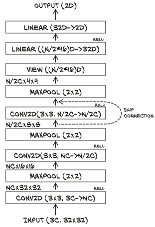
☝️ A skip connection is nothing but the addition of the input to the output of a block of layers.
Let’s add one layer to our simple convolutional model, and let’s use ReLU as the activation for a change. The vanilla module with an extra layer looks like this:
class NetDepth(nn.Module):
    def __init__(self, n_chans1=32):
        super().__init__()
        self.n_chans1 = n_chans1
        self.conv1 = nn.Conv2d(3, n_chans1, kernel_size=3, padding=1)
        self.conv2 = nn.Conv2d(n_chans1, n_chans1 // 2,
                               kernel_size=3, padding=1)
        self.conv3 = nn.Conv2d(n_chans1 // 2, n_chans1 // 2,
                               kernel_size=3, padding=1)
        self.fc1 = nn.Linear(4 * 4 * n_chans1 // 2, 32)
        self.fc2 = nn.Linear(32, 2)

    def forward(self, x):
        out = F.max_pool2d(torch.relu(self.conv1(x)), 2)
        out = F.max_pool2d(torch.relu(self.conv2(out)), 2)
        out = F.max_pool2d(torch.relu(self.conv3(out)), 2)
        out = out.view(-1, 4 * 4 * self.n_chans1 // 2)
        out = torch.relu(self.fc1(out))
        out = self.fc2(out)
        return out
Adding a skip connection a la ResNet to this model amounts to adding the output of the first layer in the forward function to the input of the third layer:
class NetRes(nn.Module):
    def __init__(self, n_chans1=32):
        super().__init__()
        self.n_chans1 = n_chans1
        self.conv1 = nn.Conv2d(3, n_chans1, kernel_size=3, padding=1)
        self.conv2 = nn.Conv2d(n_chans1, n_chans1 // 2,
                               kernel_size=3, padding=1)
        self.conv3 = nn.Conv2d(n_chans1 // 2, n_chans1 // 2,
                               kernel_size=3, padding=1)
        self.fc1 = nn.Linear(4 * 4 * n_chans1 // 2, 32)
        self.fc2 = nn.Linear(32, 2)

    def forward(self, x):
        out = F.max_pool2d(torch.relu(self.conv1(x)), 2)
        out = F.max_pool2d(torch.relu(self.conv2(out)), 2)
        out1 = out

        # Adding a skip connection is
        # adding the output of the first layer in the forward function
        # to the input of the third layer
        out = F.max_pool2d(torch.relu(self.conv3(out)) + out1, 2)

        out = out.view(-1, 4 * 4 * self.n_chans1 // 2)
        out = torch.relu(self.fc1(out))
        out = self.fc2(out)
        return out
In other words, we’re using the output of the first activations as inputs to the last, in addition to the standard feed-forward path. This is also referred to as identity mapping.
Generally speaking: just arithmetically add earlier intermediate outputs to downstream intermediate outputs.
How does this alleviate the issues with vanishing gradients?
Thinking about backpropagation, a skip connection, or a sequence of skip connections in a deep network, creates a direct path from the deeper parameters to the loss. This makes their contribution to the gradient of the loss more direct, as partial derivatives of the loss with respect to those parameters have a chance not to be multiplied by a long chain of other operations.
It has been observed that skip connections have a beneficial effect on convergence especially in the initial phases of training. Also, the loss landscape of deep residual networks is a lot smoother than feed-forward networks of the same depth and width.👏
Building very deep models in Pytorch
The standard strategy is:
define a building block, such as a
(Conv2d, ReLU, Conv2d) + skip connectionblockbuild the network dynamically in a
forloop.
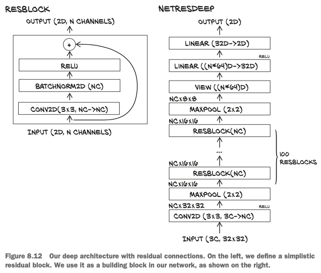
We first create a module subclass whose sole job is to provide the computation for one block—that is, one group of convolutions, activation, and skip connection:
class ResBlock(nn.Module):
    def __init__(self, n_chans):
        super(ResBlock, self).__init__()
        self.conv = nn.Conv2d(n_chans, n_chans, kernel_size=3,
                              padding=1, bias=False)
        self.batch_norm = nn.BatchNorm2d(num_features=n_chans)

        # Use custom initializations as in the ResNet paer
        torch.nn.init.kaiming_normal_(self.conv.weight, nonlinearity='relu')

        # The batch norm is initialized to produce output distributions
        # that initially have 0 mean and 0.5 variance
        torch.nn.init.constant_(self.batch_norm.weight, 0.5)
        torch.nn.init.zeros_(self.batch_norm.bias)

    def forward(self, x):
        out = self.conv(x)
        out = self.batch_norm(out)
        out = torch.relu(out)
        return out
We’d now like to generate a 100-block network.
- First, in
init, we createnn.Sequentialcontaining a list ofResBlockinstances.nn.Sequentialwill ensure that the output of one block is used as input to the next. It will also ensure that all the parameters in the block are visible toNet. - Then, in
forward, we just call the sequential to traverse the 100 blocks and generate the output
class NetResDeep(nn.Module):
    def __init__(self, n_chans1=32, n_blocks=10):
        super().__init__()
        self.n_chans1 =n_chans1
        self.conv1 = nn.Conv2d(3, n_chans1, kernel_size=3, padding=1)

        # create a list of ResBlocks
        self.resblocks = nn.Sequential(* (n_blocks * [ResBlock(n_chans=n_chans)]))

        self.fc1 = nn.Linear(8 * 8 * n_chans1, 32)
        self.fc2 = nn.Linear(32, 2)

    def forward(self, x):
        out = F.max_pool2d(torch.relu(self.conv1(x)), 2)

        # traverse the list of blocks
        out = self.resblocks(out)

        out = F.max_pool2d(out, 2)
        out = out.veiw(-1, 8 * 8 * self.n_chans1)
        out = torch.relu(self.fc1(out))
        out = self.fc2(out)
        return out