Autograd
TL;DR
- Only Tensors with
is_leaf=Trueandrequires_grad=Truecan get automatically computed gradient when callingbackward().- The gradient is stored in Tensor’s
gradattribute
- The gradient is stored in Tensor’s
- When calling
backward(), we must specify a gradient argument that is a tensor of matching shape
Overview
import torch
autograd package
- provides automatic differentiation for all operations on Tensors
- define-by-run framework
- i.e., backprop is defined by how your code is run, and that every single iteration can be different.
Dynamic Computational Graph (DCG)
Gradient enabled tensors (variables) along with functions (operations) combine to create the dynamic computational graph.
The flow of data and the operations applied to the data are defined at runtime hence constructing the computational graph dynamically. This graph is made dynamically by the autograd class under the hood.
For example,
x = torch.tensor(1.0)
y = torch.tensor(2.0)
z = x * y
The code above creates the following DCG under the hood:
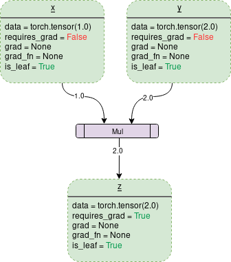
Each dotted outline box in the graph is a tensor (variable) and the purple rectangular box is an operation.
Tensor
Attributes of a tensor related to autograd are
data: data the tensor is holdingrequires_grad: if true, then starts tracking all the operation history and forms a backward graph for gradient calculation.By default is
FalseSet to
TrueDirectly set to
Truex.requires_grad = TrueOr call
.requires_grad_(True)
a = torch.randn(2, 2)
a = ((a * 3) / (a - 1))
print(a.requires_grad) # should be False if we haven't specified

# Now we set requires_grad to True explicitly
a.requires_grad_(True)
print(a.requires_grad) # Now is true
grad: holds the value of gradient- If
requires_gradis False it will hold a None value. - Even if
requires_gradis True, it will hold a None value unless.backward()function is called from some other node.
- If
grad_fn: references aFunctionthat has created theTensor(except for Tensors created by the user).b = a * a print(b.grad_fn)<MulBackward0 object at 0x7f9c18a5b3c8>is_leaf: a node is leaf ifIt was initialized explicitly by some functions, e.g.
x = torch.tensor(1.0)It is created after operations on tensors which all have
requires_grad = FalseIt is created by calling
.detach()method on some tensor.
If we do NOT require gradient tracking for a tensor:
To stop a tensor from tracking history, call
.detach()to detach it from the computation history- Alternatives:
.numpy().item().tolist()(if not a scalar)
- Alternatives:
Or use call
.requires_grad_()to change an existing Tensor’srequires_gradflag toFalsein-place (The input flag defaults toFalseif not given.)To prevent tracking history (and using memory) and make the code run faster whenever gradient tracking is not needed, wrap the code block in with
torch.no_grad():with torch.no_grad(): # operations that do not need gradient tracking
backward() and Gradient Computation
On calling backward(), gradients are populated only for the nodes which have both requires_grad and is_leaf True. Gradients are of the output node from which .backward() is called, w.r.t other leaf nodes.
On turning requires_grad = True :
x = torch.Tensor(1.0, requires_grad=True)
y = torch.Tensor(2.0)
z = x * y

z.backward()
PyTorch will start tracking the operation and store the gradient functions at each step as follows:
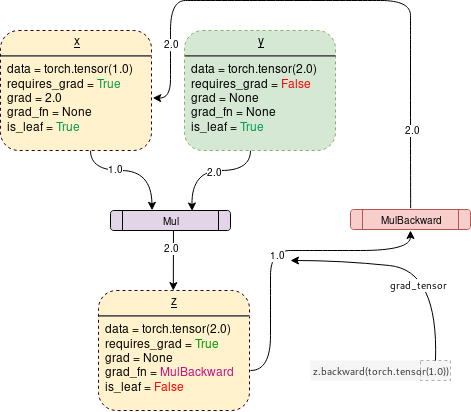
- Leaf nodes:
x: Asrequires_grad=True, its gradient ($\frac{\partial z}{\partial x}$) will be computed when callingbackward()and the gradient will be stored inx’sgradattributey:requires_grad=False, thus its gradient won’t be computed andgradis none
- Branch node
z(“branch” means non-leaf)x, one of the tensors that createz, hasrequires_grad=True. Thereforezalso hasrequires_grad=Truezis the result of multiplication operation. Therefore itsgrad_fnrefers toMulBackward
backward() is the function which actually calculates the gradient by passing it’s argument (1x1 unit tensor by default) through the backward graph all the way up to every leaf node traceable from the calling root tensor. The calculated gradients are then stored in .grad of every leaf node.
grad_tensor
An important thing to notice is that when z.backward() is called, a tensor is automatically passed as z.backward(torch.tensor(1.0)). The torch.tensor(1.0) is the external gradient (the grad_tensor) provided to terminate the chain rule gradient multiplications. This external gradient is passed as the input to the MulBackward function to further calculate the gradient of x.
The dimension of tensor passed into .backward() must be the same as the dimension of the tensor whose gradient is being calculated.
Contains only one element (i.e. scalar)
If the result Tensor is a scalar (i.e. it holds a one element data), we don’t need to specify any arguments to backward(). For example:
a = torch.tensor(1.0, requires_grad=True) # a is a scalar
b = a + 2
c = a * b # c is also a scalar

c.backward()
print(a.grad)
tensor(4.)
Contains more than one element
If result Tensor has more elements, we need to specify a gradient argument that is a tensor of matching shape. For example:
x = torch.ones(3, requires_grad=True)

def f(x):
  y = x * 2
  z = y * y * 2
  return z

print(f"f(x): {f(x)}") # f(x) is a vector, not a scalar
f(x): tensor([8., 8., 8.], grad_fn=<MulBackward0>)
Now in this case z is no longer a scalar. torch.autograd could not compute the full Jacobian directly, but if we just want the vector-Jacobian product, simply pass the vector to backward as argument:
v = torch.tensor([1, 2, 3], dtype=torch.float)
f(x).backward(v, retain_graph=True)
# alternatively we can call static backward in autograd package as following:
# torch.autograd.backward(z, grad_tensors=v, retain_graph=True)

print(f"gradint of x: {x.grad}")
gradint of x: tensor([16., 32., 48.])
$$ > f(x) = 8x^2 = (8x_1^2 \quad 8x_2^2 \quad 8x_3^2)^T > $$ $$ > J = \frac{\partial f}{\partial x} = \left(\begin{array}{ccc} > \frac{\partial f\_{1}}{\partial x\_{1}} & \frac{\partial f\_{1}}{\partial x\_{2}} & \frac{\partial f\_{1}}{\partial x\_{3}}\\\\ > \frac{\partial f\_{2}}{\partial x\_{1}} & \frac{\partial f\_{2}}{\partial x\_{2}} & \frac{\partial f\_{2}}{\partial x\_{3}}\\\\ > \frac{\partial f\_{3}}{\partial x\_{1}} & \frac{\partial f\_{3}}{\partial x\_{2}} & \frac{\partial f\_{3}}{\partial x\_{3}} > \end{array}\right)= \left(\begin{array}{ccc} > 16 & 0 & 0\\\\ > 0 & 16 & 0\\\\ > 0 & 0 & 16 > \end{array}\right) > $$ $$ > v = (\frac{\partial l}{\partial y\_1} \quad \frac{\partial l}{\partial y\_2} \quad \frac{\partial l}{\partial y\_3})^T =: (1 \quad 2 \quad 3)^T > $$ $$ > v^T \cdot J = (\frac{\partial l}{\partial x\_1} \quad \frac{\partial l}{\partial x\_2} \quad \frac{\partial l}{\partial x\_3})^T = (1 \quad 2 \quad 3) \left(\begin{array}{ccc} > 16 & 0 & 0\\\\ > 0 & 16 & 0\\\\ > 0 & 0 & 16 > \end{array}\right) = (16 \quad 32 \quad 48) > $$
If we want to compute $\frac{\partial f}{\partial x}$, simply pass the unit tensor (all elements are 1) of the matching shape as grad_tensor:
x.grad.zero_() # clear previous gradient otherwise it will get accumulated
unit_tensor = torch.ones(3, dtype=torch.float)
f(x).backward(unit_tensor, retain_graph=True)
print(f"gradint of x: {x.grad}")
gradint of x: tensor([16., 16., 16.])
The tensor passed into the backward function acts like weights for a weighted output of gradient. Mathematically, this is the vector multiplied by the Jacobian matrix of non-scalar tensors (discussed in Appendix). Hence it should almost always be a unit tensor of dimension same as the tensor backward is called upon, unless weighted outputs needs to be calculated.
Video Tutorial
Great explanation, highly recommend! 🔥
Appendix
Generally speaking, torch.autograd is an engine for computing
vector-Jacobian product. That is, given any vector
$$ v=\left(\begin{array}{cccc} v\_{1} & v\_{2} & \cdots & v\_{m}\end{array}\right)^{T} $$compute the product $v^{T}\cdot J$.
If $v$ happens to be the gradient of a scalar function $l=g\left(\vec{y}\right)$, that is,
$$ v=\left(\begin{array}{ccc}\frac{\partial l}{\partial y_{1}} & \cdots & \frac{\partial l}{\partial y_{m}}\end{array}\right)^{T} $$then by the chain rule, the vector-Jacobian product would be the gradient of $l$ with respect to $\vec{x}$:
$$ \begin{align}J^{T}\cdot v=\left(\begin{array}{ccc} \frac{\partial y\_{1}}{\partial x\_{1}} & \cdots & \frac{\partial y\_{m}}{\partial x\_{1}}\\\\ \vdots & \ddots & \vdots\\\\ \frac{\partial y\_{1}}{\partial x\_{n}} & \cdots & \frac{\partial y\_{m}}{\partial x\_{n}} \end{array}\right)\left(\begin{array}{c} \frac{\partial l}{\partial y\_{1}}\\\\ \vdots\\\\ \frac{\partial l}{\partial y\_{m}} \end{array}\right)=\left(\begin{array}{c} \frac{\partial l}{\partial x\_{1}}\\\\ \vdots\\\\ \frac{\partial l}{\partial x\_{n}} \end{array}\right) \end{align} $$(Note that $v^{T}\cdot J$ gives a row vector which can be treated as a column vector by taking $J^{T}\cdot v$.)
This characteristic of vector-Jacobian product makes it very convenient to feed external gradients into a model that has non-scalar output. 👏