Prädiktion nichtlinearer Systeme
Chapman-Kolmogorov-Gleichung
Verbunddichte
$$ f\left(\underline{x}_{k+1}, \underline{x}_{k}\right)=f\left(\underline{x}_{k+1} \mid \underline{x}_{k}\right) \cdot f\left(\underline{x}_{k}\right) $$Marginalisierung
$$ f\left(x_{k+1}\right)=\int_{\mathbb{R}^{N}} f\left(\underline{x}_{k+1} \mid \underline{x}_{k}\right) \cdot f\left(\underline{x}_{k}\right) d \underline{x}_{k} $$Definition
geschätzte Dichte im Zeitschritt $k$ einschließlich der letzten Messung
$$ f_{k}^{e}\left(\underline{x}_{k}\right)=f\left(\underline{x}_{k} \mid \underline{\hat{y}}_{k}, \underline{\hat{y}}_{k-1}, \ldots, \underline{\hat{y}}_{1}, \underline{\hat{u}}_{k-1}, \underline{\hat{u}}_{k-2}, \ldots, \underline{\hat{u}}_{0}\right) $$Prädiktion der Dichte im Zeitschritt $k+1$ (Messung nicht inklusive)
$$ f_{k+1}^{p}\left(\underline{x}_{k+1}\right)=f\left(\underline{x}_{k+1} \mid \underline{\hat{y}}_{k}, \underline{\hat{y}}_{k-1}, \ldots, \underline{\hat{y}}_{1}, \underline{\hat{u}}_{k}, \underline{\hat{u}}_{k-1}, \ldots, \underline{\hat{u}}_{0}\right) $$
Prädiktion für dynamische Systeme ( Chapman-Kolmogorov-Gleichung)
$$ f_{k+1}^{p}\left(\underline{x}_{k+1}\right)=\int_{\mathbb{R}^{N}} \underbrace{f\left(\underline{x}_{k+1} \mid \underline{x}_{k}\right)}_{\text{Prädiktionsdichte}} f_{k}^{e}\left(\underline{x}_{k}\right) \mathrm{d} \underline{x}_{k} $$Erklärung
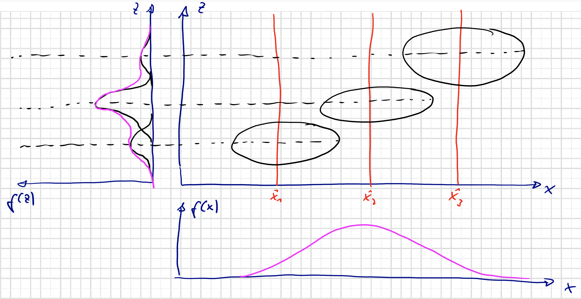
Die Chapman-Kolmogorov-Gleichung berechnet die Dichte von $\underline{x}_{k+1}$ aus einer gegebenen Dichte $f_{k}^{e}\left(\underline{x}_{k}\right)$ von $\underline{x}_{k}$ , während die probabilistische Systembeschreibung $f\left(\underline{x}_{k+1} \mid \underline{x}_{k}\right)$ die Dichte von $\underline{x}_{k+1}$ für einen konkreten Wert von $\underline{x}_{k}$ aus.
- $f\left(\underline{x}_{k+1} \mid \underline{x}_{k}\right)$
das probablistische Systemmodell, welches eine Wahrscheinlichkeitsdichte für den nächsten Zustand $\underline{x}_{k+1}$ zu einem gegebenen aktuellen Zustand $\underline{x}_{k}$ ausgibt.
Diese Transitionsdichte $f\left(\underline{x}_{k+1} \mid \underline{x}_{k}\right)$ können wir aus dem gegebenen Systemmodell $\underline{x}_{k+1} = \underline{a}(\underline{x}_{k}, \underline{u}_{k}, \underline{v}_{k})$ berechnen - es ist einfach die probabilistische Darstellung davon
$$ f\left(\underline{x}_{k+1} \mid \underline{x}_{k}\right) = \int_{\mathbb{R}^N} \delta(\underline{x}_{k+1} - \underline{a}(\underline{x}_{k}, \underline{u}_{k}, \underline{v}_{k})) \cdot f_k^v(\underline{v}_k) d \underline{v}_k $$
- $f_{k}^{e}\left(\underline{x}_{k}\right)$
die beste Schätzung, die wir über den Systemzustand zum Zeitpunkt $k$ haben, gegeben als Wahrscheinlichkeitsdichte
- $f_{k+1}^{p}\left(\underline{x}_{k+1}\right)$
- die beste Prädiktion des Zustands zum Zeitpunkt $(k+1)$, die sich aus dem Wissen über den Zustand $f_{k}^{e}\left(\underline{x}_{k}\right)$ und dem Systemmodell $\underline{x}_{k+1} = \underline{a}(\underline{x}_{k}, \underline{u}_{k}, \underline{v}_{k})$ (generative Darstellung) bzw. $f\left(\underline{x}_{k+1} \mid \underline{x}_{k}\right)$ (probabilistische Darstellung) berechnen lässt.
- Bei einer Prädiktion wird die (relative) Unsicherheit generell größer.
Problem
‼️ Es handelt sich um ein Parameterintegral!
- Integrand hängt von $\underline{x}_{k+1}$ ab (lässt sich i.Allg nicht herausziehen)
- Nur möglich für analytische Lösung
- Sonst erfordert (numerische) Lösung des Integrals für alle $\underline{x}_{k+1}$
Weiter nützliche Form der CK-Gleichung
$$ \begin{aligned} f(\underline{x}_{k + 2}, \underline{x}_{k}) &= \int_{\mathbb{R}^N} f(\underline{x}_{k+2}, \underline{x}_{k+1}, \underline{x}_{k}) d\underline{x}_{k+1} \\\\ f(\underline{x}_{k + 2} \mid \underline{x}_{k}) f(\underline{x}_{k}) &= \int_{\mathbb{R}^N} f(\underline{x}_{k+2} \mid \underline{x}_{k+1}, \underline{x}_{k}) f(\underline{x}_{k+1}, \underline{x}_{k}) d\underline{x}_{k+1} \quad | \quad \text{Markov} \\\\ f(\underline{x}_{k + 2} \mid \underline{x}_{k}) f(\underline{x}_{k}) &= \int_{\mathbb{R}^N} f(\underline{x}_{k+2} \mid \underline{x}_{k+1}) f(\underline{x}_{k+1}, \underline{x}_{k}) d\underline{x}_{k+1} \\\\ f(\underline{x}_{k + 2} \mid \underline{x}_{k}) f(\underline{x}_{k}) &= \int_{\mathbb{R}^N} f(\underline{x}_{k+2} \mid \underline{x}_{k+1}) f(\underline{x}_{k+1} \mid \underline{x}_{k}) f(\underline{x}_{k})d\underline{x}_{k+1} \\\\ f(\underline{x}_{k + 2} \mid \underline{x}_{k}) &= \int_{\mathbb{R}^N} f(\underline{x}_{k+2} \mid \underline{x}_{k+1}) f(\underline{x}_{k+1} \mid \underline{x}_{k}) d\underline{x}_{k+1} \end{aligned} $$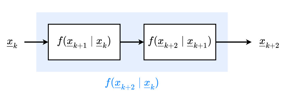
Prädiktion mit CK-Glg.: Lösungsansätze
Im allgemeinen Fall ist CK-Gleichung NICHT exakt lösbar 🤪
Ausnahme (Bsp.)
System ist linear und $f_{k}^{e}(\cdot)$ kann durch erste zwei Momente beschrieben werden
$f_{k}^{e}(\underline{x}_k)$ ist durch Abstastwerte repräsentiert.
$$ \begin{aligned} & f_{k}^{e}\left(\underline{x}_{k}\right)=\sum_{i=1}^{L} w_{i} \delta\left(\underline{x}_{k}-\hat{\underline{x}}_{k, i}\right) \qquad w_i \geq 0, \sum_i w_i = 1\\ \Rightarrow \qquad & f_{k=1}^{p}\left(\underline{x}_{k+1}\right)=\sum_{i=1}^{L} w_{i} f\left(\underline{x}_{k+1} \mid \hat{\underline{x}}_{k, i}\right) \end{aligned} $$
Vereinfachte Prädiktion
Systemmodell mit additivem Rauschen
Wir beginnen mit additivem Rauschen.
Generatives Modell
$$ \underline{x}_{k+1} = \underline{a}_{k}(\underline{x}_{k}) + \underline{w}_{k} \qquad \underline{x}_{k+1}, \underline{x}_{k}, \underline{w}_{k} \in \mathbb{R}^N $$Vereinfachte Schreibweise
$$ \underline{z} = \underline{a}(\underline{x}) + \underline{w} $$Probablistisches Modell (inkl. Rauschen)
$$ f(\underline{z} \mid \underline{x}) = f_w(\underline{z} - \underline{a}(\underline{x})) $$Vereinfachung: Aufteilung in diskrete “Streifen”:
$$ f\left(\underline{z} \mid \underline{\hat{x}}_{i}\right)=f_w\left(\underline{z}-\underline{a}\left(\underline{\hat{x}}_{i}\right)\right) \qquad i \in \mathbb{Z} $$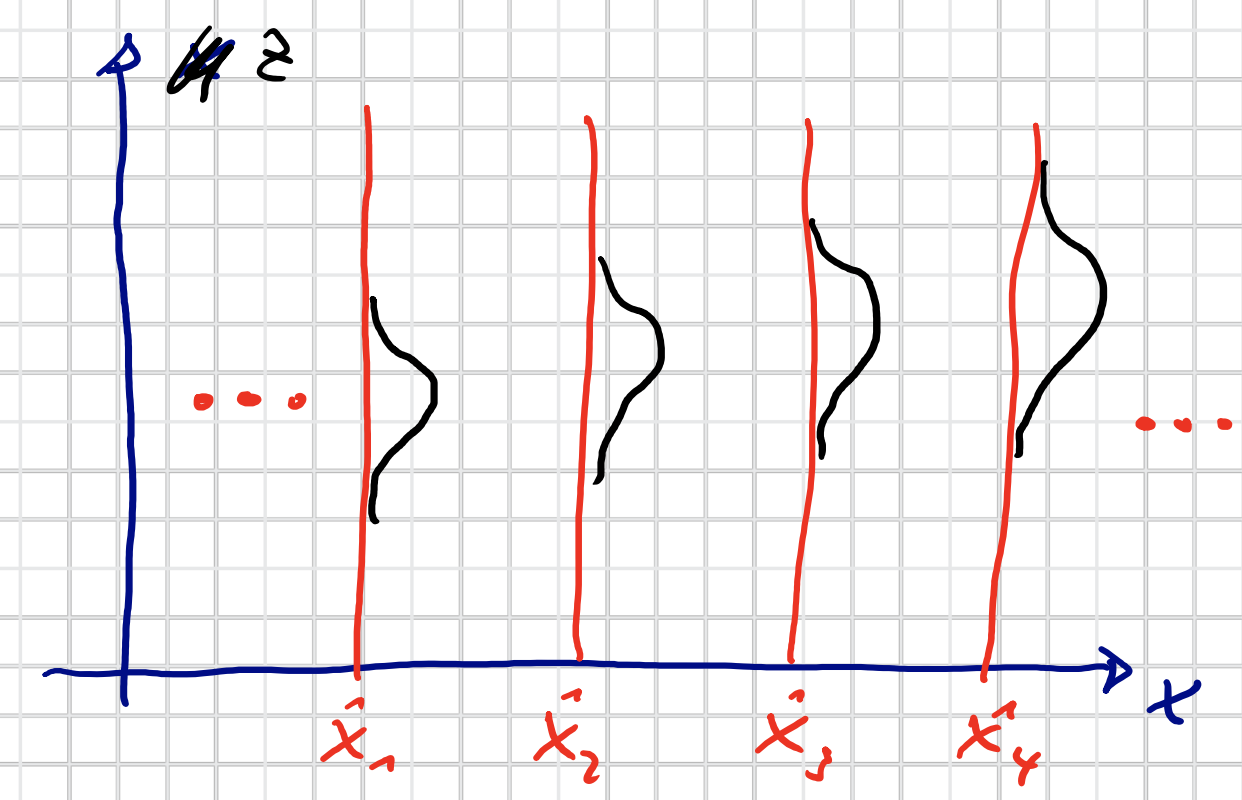
In den “Zwischenräumen” gilt nun aber $\int f(\underline{z} \mid \underline{x}) = 1$ NICHT. Wir definiere eine “Füllfunktion” $f_i(\underline{x})$:
$$ f_i(\underline{x}) = \mathcal{N}(\underline{x}, \underline{\hat{x}}_i, C_i) \qquad i \in \mathbb{Z} $$mit
$$ f(\underline{x}) = \sum_{i \in \mathbb{Z}} w_if_i(\underline{x}) \approx 1 $$Z.B. Skalarer Fall
$$ > f(x)=\sum_{i \in \mathbb{Z}} w_{i} f_i(x), \quad f_i(x)=\exp \left(-\frac{1}{2} \frac{\left(x-\hat{x}_{i}\right)^{2}}{\sigma^{2}}\right) > $$mit geeigneten $\sigma$.
Betrachtung für jeweils ein Komponente $i$
$$ f_i(\underline{z} \mid \underline{x}) = f(\underline{z} \mid \underline{\hat{x}}_i) \cdot f_i(\underline{x}) $$Gesamtdichte ist
$$ f(\underline{z} \mid \underline{x}) \approx \sum_{i \in \mathbb{Z}} w_i f(\underline{z} \mid \underline{\hat{x}}_i) \cdot f_i(\underline{x}) $$Es gilt
$$ \begin{aligned} \int_{\mathbb{R}^{N}} f(\underline{z}(\underline{x}) d \underline{z}&=\sum_{i \in \mathbb{Z}} w_{i} f_{i}(\underline{x}) \underbrace{\int_{\mathbb{R}^N}f(\underline{z} \mid \underline{x}) d\underline{z}}_{=1}\\ &=\sum_{i \in \mathbb{Z}} w_{i} f_{i}(\underline{x}) \approx 1 \end{aligned} $$Fall Rauschen $\underline{w}_k$ Gaußverteilt, ist $f(\underline{z} \mid \underline{x} )$ Gaussian Mixture
$$ f(\underline{z} \mid \underline{x}) = \sum_{i \in \mathbb{Z}} \underbrace{f_i^z(\underline{z})}_{f_w(\underline{z} - \underline{a}(\underline{\hat{x}}_i))} \cdot f_i^x(\underline{x}) $$Allgemeine Systemmodelle
$$ \underline{x}_{k+1} = \underline{a}_k (\underline{x}_k, \underline{w}_k) $$Vereinfachte Schreibweise:
$$ \underline{z} = \underline{a}(\underline{x}, \underline{w}) $$Ergibt allgemeine Transitionsdichte $f(\underline{z} | \underline{x})$, auch durch Mixture approximierbar
$$ f(\underline{z} | \underline{x}) = \sum_{i \in \mathbb{Z}} w_i f_i^z(\underline{z}) \cdot f_i^x(\underline{x}) $$
Wichtig ist, dass die einzelnen Komponenten entkoppelt sind. 👏
Bsp 1
Annahme: $f(\underline{x})$ ist eine Gaußdichte.
Einsetzen in CK-Gleichung:
$$ \begin{aligned} f(\underline{z})&=\int_{\mathbb{R}^{N}}\left(\sum_{i \in \mathbb{Z}} w_{i} f_{i}^{z}(\underline{z}) \cdot f_{i}^{x}(\underline{x})\right) f(\underline{x}) d \underline{x}\\ &=\sum_{i \in \mathbb{Z}} w_{i} f_{i}^{z}(\underline{z}) \underbrace{\int_{\mathbb{R}^{N}} f_{i}^{x}(\underline{x}) \cdot f(\underline{x}) d \underline{x}}_{\text{Konstante } c_{i}}\\ &= \sum_{i \in \mathbb{Z}} \underbrace{w_{i} c_i}_{=: \bar{w}_i} f_{i}^{z}(\underline{z})\\ &=\sum_{i \in \mathbb{Z}} \bar{w}_{i} f_{i}^{z}(\underline{z}) \end{aligned} $$Hier sieht man, dass $f_i^z(\underline{z})$ einfach aus dem Integral ausgezogen werden kann. Innerhalb des Integrals gibt es nur $\underline{x}$.
Speizialfall: $f(\underline{x}) = \delta(\underline{x} - \underline{\hat{x}}) \Rightarrow$
$$ c_i = \int_{\mathbb{R}^{N}} f_{i}(\underline{x}) \delta \left(\underline{x}-\underline{\hat{x}}\right) d \underline{x}=f_i(\underline{\hat{x}}) $$Bsp 2
Annahme: Gaussian Mixture
$$ f(\underline{x}) = \sum_{j=1}^L v_j f_j^*(\underline{x}) $$Einsetzen in CK-Gleichung:
$$ \begin{aligned} f(\underline{z})&=\int_{\mathbb{R}^{N}}\left\{\sum_{i \in \mathbb{Z}} w_{i} f_{i}^{z}(\underline{z}) f_{i}^{x}(\underline{x})\right\} \cdot \left\{\sum_{i=1}^{L} v_{j} f_{j}^{*}(\underline{x})\right\} d x\\ &=\sum_{i \in \mathbb{Z}} w_{i} f_{i}^{z}(\underline{z}) \underbrace{\sum_{i=1}^{L} v_{j} \underbrace{\int_{\mathbb{R}^N} f_{i}^{x}(\underline{x}) \cdot f_{j}^{*}(\underline{x}) d \underline{x}}_{\text{Konstante}}}_{\text {Kondante } C_{i}} \\ &=\sum_{i \in \pi} \underbrace{w_{i}C_i}_{=: \bar{w}_i} f_{i}^{z}(\underline{z}) \\ &=\sum_{i \in \pi} \bar{w}_{i} f_{i}^{z}(\underline{z}) \end{aligned} $$